1.1.2 A First Regression
A fit is the result of solving an optimization problem on a dataset. For a Gaussian model, the objective described in the R glmnet vignette is:
minβ₀,β 1/(2n) ∑ᵢ₌₁ⁿ (yᵢ − β₀ − xᵢᵀβ)² + λ [α‖β‖₁ + (1−α)/2 ‖β‖₂²]
The solution gives the intercept β₀ and the predictor coefficients β. Each of the n observations has predictors xᵢ and a response yᵢ. The penalty’s strength is λ ≥ 0, and α ∈ [0, 1] mixes the lasso and ridge penalties. Ordinary least squares (OLS) sets λ = 0; see The penalty: α and λ for the other choices.
R’s mtcars dataset measures 32 cars. Load it as a Polars dataframe:
> (require datasets) > (define cars (load-dataset 'mtcars #:format 'polars)) > cars
shape: (32, 12)
┌───────────────────┬──────┬─────┬───────┬───┬─────┬─────┬──────┬──────┐
│ model ┆ mpg ┆ cyl ┆ disp ┆ … ┆ vs ┆ am ┆ gear ┆ carb │
│ --- ┆ --- ┆ --- ┆ --- ┆ ┆ --- ┆ --- ┆ --- ┆ --- │
│ str ┆ f64 ┆ i64 ┆ f64 ┆ ┆ i64 ┆ i64 ┆ i64 ┆ i64 │
╞═══════════════════╪══════╪═════╪═══════╪═══╪═════╪═════╪══════╪══════╡
│ Mazda RX4 ┆ 21.0 ┆ 6 ┆ 160.0 ┆ … ┆ 0 ┆ 1 ┆ 4 ┆ 4 │
│ Mazda RX4 Wag ┆ 21.0 ┆ 6 ┆ 160.0 ┆ … ┆ 0 ┆ 1 ┆ 4 ┆ 4 │
│ Datsun 710 ┆ 22.8 ┆ 4 ┆ 108.0 ┆ … ┆ 1 ┆ 1 ┆ 4 ┆ 1 │
│ Hornet 4 Drive ┆ 21.4 ┆ 6 ┆ 258.0 ┆ … ┆ 1 ┆ 0 ┆ 3 ┆ 1 │
│ Hornet Sportabout ┆ 18.7 ┆ 8 ┆ 360.0 ┆ … ┆ 0 ┆ 0 ┆ 3 ┆ 2 │
│ … ┆ … ┆ … ┆ … ┆ … ┆ … ┆ … ┆ … ┆ … │
│ Lotus Europa ┆ 30.4 ┆ 4 ┆ 95.1 ┆ … ┆ 1 ┆ 1 ┆ 5 ┆ 2 │
│ Ford Pantera L ┆ 15.8 ┆ 8 ┆ 351.0 ┆ … ┆ 0 ┆ 1 ┆ 5 ┆ 4 │
│ Ferrari Dino ┆ 19.7 ┆ 6 ┆ 145.0 ┆ … ┆ 0 ┆ 1 ┆ 5 ┆ 6 │
│ Maserati Bora ┆ 15.0 ┆ 8 ┆ 301.0 ┆ … ┆ 0 ┆ 1 ┆ 5 ┆ 8 │
│ Volvo 142E ┆ 21.4 ┆ 4 ┆ 121.0 ┆ … ┆ 1 ┆ 1 ┆ 4 ┆ 2 │
└───────────────────┴──────┴─────┴───────┴───┴─────┴─────┴──────┴──────┘
Predict fuel economy (mpg, miles per US gallon) from weight (wt, in thousands of pounds) and horsepower (hp). ols fits without a penalty; name the response column, then the predictor columns:
> (define fit (ols cars "mpg" #:predictors '("wt" "hp"))) > fit #<glmnet:gaussian λ=0 dev=0.8268 nz=2/2>
> (coef fit) '#(37.22729275591213 -3.8778430581971657 -0.03177283120189043)
The fit prints its family, λ, the fraction of variance explained (R²) and how many coefficients are nonzero. coef gives the intercept, then one coefficient per predictor, in the order named. Name them with match-define:
> (match-define (vector β₀ β-wt β-hp) (coef fit)) > (~r (* 100 β-hp) #:precision 2) "-3.18"
> (deviance-ratio fit) 0.8267854518805285
(* 100 β-hp) is the change in predicted fuel economy for 100 more horsepower at the same weight. deviance-ratio is R².
A penalty shrinks the coefficients. lasso applies the L1 penalty, which can set coefficients to zero; at λ = 4 it drops horsepower:
> (define penalized-fit (lasso cars "mpg" #:predictors '("wt" "hp") #:lambda 4.0)) > (coef penalized-fit) '#(23.92234052081157 -1.1909909148532365 0.0)
A regularization path fits many values of λ at once. elnet-path uses the lasso penalty by default. Its summary shows, for each λ, the number of nonzero coefficients and the percentage of deviance explained:
> (elnet-path cars "mpg" #:predictors '("wt" "hp") #:nlambda 12)
#<glmnet-path:gaussian
Df %Dev Lambda
1 0 0.00 5.1470
2 2 65.67 2.2280
3 2 79.49 0.9645
4 2 82.08 0.4175
5 2 82.57 0.1807
6 2 82.66 0.0782
7 2 82.67 0.0339
8 2 82.68 0.0147
9 2 82.68 0.0063>
1.1.2.1 Plotting the fit and path
glmnet/plot draws coefficient paths and cross-validation curves, and Racket’s plot everything else. These examples return picts, which this manual and DrRacket show as images:
> (require glmnet/plot plot (only-in polars ref series->list))
1.1.2.1.1 Predicted versus actual values
Points on the dashed line have equal predicted and actual values; points above it are underpredictions:
> (define fitted (predict fit cars)) > (define actual (series->list (ref cars "mpg")))
> (plot-pict (list (function values #:color "gray" #:style 'short-dash) (points (map vector fitted actual) #:alpha 0.5 #:size 3)) #:x-label "Predicted fuel economy (mpg)" #:y-label "Actual fuel economy (mpg)" #:title "Mtcars: OLS predicted vs actual" #:width 640 #:height 360)
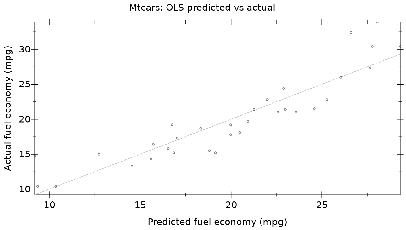
These are the cars the model was fitted to, so this plot, the next and R² describe the fit, not its error on new cars; Choosing λ by cross-validation estimates that.
1.1.2.1.2 Residuals versus fitted values
A residual is the observed response minus its fitted value, rᵢ = yᵢ − ŷᵢ:
> (plot-pict (list (hrule 0 #:color "gray" #:style 'short-dash) (points (map vector fitted (map - actual fitted)) #:alpha 0.5 #:size 3)) #:x-label "Fitted fuel economy (mpg)" #:y-label "Residual (observed - fitted)" #:title "Mtcars: OLS residuals vs fitted" #:width 640 #:height 360)
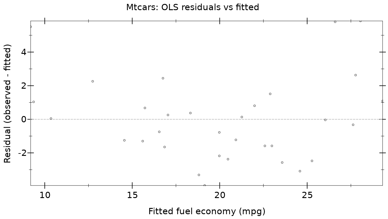
Curvature suggests a missing nonlinear term; a widening spread suggests that the variance changes with the fitted response.
1.1.2.1.3 The lasso coefficient path
> (plot-coefficient-path (elnet-path cars "mpg" #:predictors '("wt" "hp")) #:label #t #:width 640 #:height 360 #:title "Mtcars: lasso coefficient path")
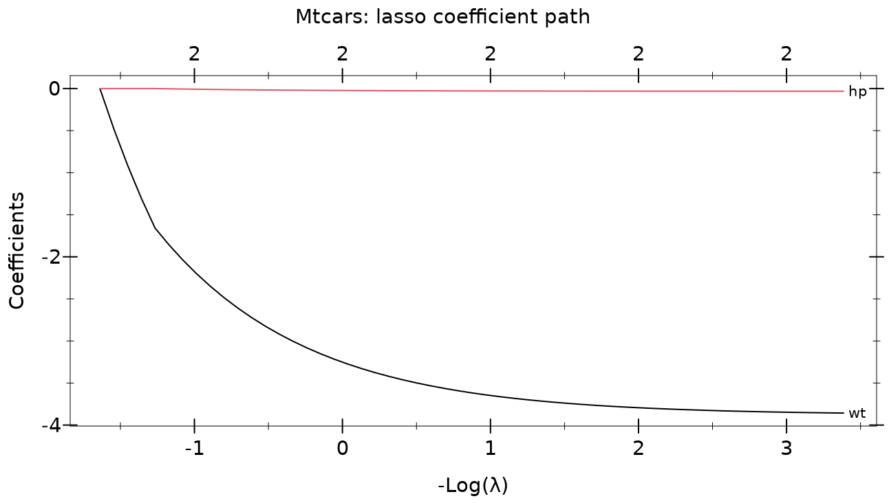
Each curve is a predictor’s coefficient, labelled with its name, as the penalty weakens from left to right. The horizontal axis is −log λ; the top axis counts the nonzero coefficients. See Plots for the other plots.
1.1.2.2 Choosing λ by cross-validation
elnet-cv cross-validates a path: it fits the path without each fold of cars in turn and measures the error of predicting the fold. Fixed fold ids make the result repeatable:
> (define cv (elnet-cv cars "mpg" #:predictors '("wt" "hp") #:fold-ids (for/list ([i 32]) (modulo i 8)))) > cv
#<glmnet-cv:gaussian
Measure: Mean-Squared Error
Lambda Index Measure SE Nonzero
min 0.0339 55 8.246 2.061 2
1se 1.1617 17 10.168 3.016 2>
> (glmnet-cv-lambda-min cv) 0.033863698479201315
> (glmnet-cv-lambda-1se cv) 1.161683775539293
lambda-min has the smallest cross-validated error; lambda-1se, the default for coef and predict on cv, is the largest λ within one standard error of it. plot-cv draws the error curve, with the two marked:
> (plot-cv cv #:width 640 #:height 360 #:title "Mtcars: cross-validated error")
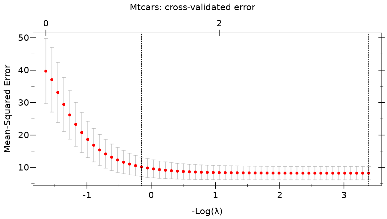
Concepts covers folds and error measures.