6 Data wrangling, 101

6 Data wrangling, 101🔗ℹ

Graphite does some of the work for us with regards to data processing. Note the 'count and 'prop modes in the earlier bar charts: we didn’t have to handle that. But Graphite is not a data wrangling library, and oftentimes it makes more sense to process our data first.

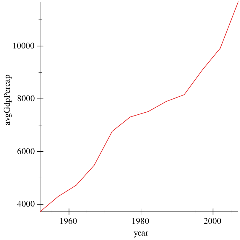
For example, in the last example, we got GDP per capita summary statistics for each continent. But what if we want the average, global GDP per capita over time? That’s too complex of a transformation for Graphite to do for us.

For this purpose, we need the Sawzall library, whose documentation is available at Sawzall: A grammar for chopping up data. This library is designed to take in data-frames, and produce new ones with some transformation applied – with operations chaining together using the threading library.

Let’s say we want to perform the above transformation on the Gapminder dataset. Effectively, what we want to do is:

Take all the data in each year, ignoring country,
average the GDP per capita within each year,
then collect the results of that sum into a new data-frame.

This translates naturally to the following Sawzall pipeline:

> (define (sum vec) (for/sum ([v (in-vector vec)]) v))
> (define (avg vec) (/ (sum vec) (vector-length vec)))
> (~> gapminder
      (group-with "year")
      (aggregate [avgGdpPercap (gdpPercap) (avg gdpPercap)])
      show)
data-frame: 12 rows x 2 columns
┌──────────────────┬────┐
│avgGdpPercap      │year│
├──────────────────┼────┤
│3725.276045801409 │1952│
├──────────────────┼────┤
│4299.4083448760575│1957│
├──────────────────┼────┤
│4725.812341961976 │1962│
├──────────────────┼────┤
│5483.653046835208 │1967│
├──────────────────┼────┤
│6770.082815282392 │1972│
├──────────────────┼────┤
│7313.166420794365 │1977│
└──────────────────┴────┘
6 rows, 0 cols elided
(use (show df everything #:n-rows 'all) for full frame)

Let’s break down this code.

The ~> operator is effectively "spicy function composition"; (~> h g f x) translates at compile-time to (f (g (h x))). We use it here to express the idea of "do-this-then-that".
(group-with "year") takes gapminder, and groups it with respect to the variable "year". This tells sequential operations that we want to treat each different possibility of year seperately.
(aggregate [avgGdpPercap (gdpPercap) (avg gdpPercap)]) aggregates each group into a single value. avgGdpPercap tells us what the new column name should be, (gdpPercap) tells us that we want to bind the variable gdpPercap as a vector in the body, and (avg gdpPercap) computes the average value of each vector.
This is a lot to break down, but more or less it takes each year, gets all the GDP per capita values that correspond to it, and averages them.
This also strips down the group structure, since we now only have one row for each year.
show prints out the result, and returns nothing, being the last thing in the pipeline.

Instead of merely printing out the data, we can use _ to tell ~> where to put the next input, and feed it directly into graph, printing out a time series of global GDP per capita:

> (~> gapminder
      (group-with "year")
      (aggregate [avgGdpPercap (gdpPercap) (avg gdpPercap)])
      (graph #:data _
             #:mapping (aes #:x "year" #:y "avgGdpPercap")
             (lines)))

This works, but isn’t a very useful example, and doesn’t teach us anything about how to work with NA values, et cetera. So, for a more complex example, we’ll take a look at the GSS again. We saw already that bar can plot counts and relative frequencies. However, oftentimes it makes more sense to get the data in the shape you want it first, and then have Graphite focus its effort on plotting the data, rather than messing with it on-the-fly.

Say we want to plot the row-marginals of region within religion (so, within each region, what is the % of each religion). We start from our gss table, which has individual-level observations, and go from there. Effectively, what we want to do is:

Take our individual-level data,
group it with respect to region, and then religion within region,
summarize each religion into a count of respondents,
then calculate the percentage of each religion within region.

Once again, we’ll build a Sawzall pipeline, but this time we’ll approach it incrementally. First off, we group with respect to the variables "bigregion" and "religion". This means that the result is internally different, but the result of show does not change. It’s merely a marker to tell future operations what to do.

> (~> gss
      (group-with "bigregion" "religion")
      show)
data-frame: 2867 rows x 33 columns
groups: (religion bigregion)
┌─────┬─────────┬────┬────────┬────────┬──────┐
│grass│marital  │kids│siblings│relig   │ballot│
├─────┼─────────┼────┼────────┼────────┼──────┤
│NA   │Married  │1   │6+      │Catholic│1     │
├─────┼─────────┼────┼────────┼────────┼──────┤
│Legal│Married  │0   │4       │Catholic│3     │
├─────┼─────────┼────┼────────┼────────┼──────┤
│Legal│Married  │2   │6+      │Catholic│3     │
├─────┼─────────┼────┼────────┼────────┼──────┤
│Legal│Married  │2   │6+      │Catholic│3     │
├─────┼─────────┼────┼────────┼────────┼──────┤
│NA   │Married  │0   │2       │Catholic│1     │
├─────┼─────────┼────┼────────┼────────┼──────┤
│Legal│Separated│4+  │4       │Catholic│2     │
└─────┴─────────┴────┴────────┴────────┴──────┘
2861 rows, 27 cols elided
(use (show df everything #:n-rows 'all) for full frame)

Note that multiple arguments to group-with say "group with respect to the first, then within each possibility for the first, group with respect to the second" and so on. Successive calls to group-with do not work.

We then want to get the number of observations within each religion. Note that aggregate above bound a variable, and computed something with it. Here, we just want to compute the length of the input, so we call vector-length on whatever variable we feel like, and turn it into a new variable "count".

> (~> gss
      (group-with "bigregion" "religion")
      (aggregate [count (bigregion) (vector-length bigregion)])
      show)
data-frame: 24 rows x 3 columns
groups: (bigregion)
┌─────────┬─────┬──────────┐
│bigregion│count│religion  │
├─────────┼─────┼──────────┤
│Midwest  │172  │Catholic  │
├─────────┼─────┼──────────┤
│Midwest  │3    │Jewish    │
├─────────┼─────┼──────────┤
│Midwest  │5    │NA        │
├─────────┼─────┼──────────┤
│Midwest  │157  │None      │
├─────────┼─────┼──────────┤
│Midwest  │33   │Other     │
├─────────┼─────┼──────────┤
│Midwest  │325  │Protestant│
└─────────┴─────┴──────────┘
18 rows, 0 cols elided
(use (show df everything #:n-rows 'all) for full frame)

Note that this both removed a layer of grouping, and significantly stripped down our table. aggregate removes all columns except groups and the columns created (because where would it put the other observations?).

We then want to take this result, and then create new variables at the current level of grouping (with respect to region), telling us the percent preference by region. So, what we want to do is calculate the frequency of each religion in each region (so the count divided by the total), and then multiply it by 100 (to turn it into a percentage). We use Sawzall’s create operation for this:

> (define (v/ vec c) (vector-map (λ (x) (/ x c)) vec))
> (~> gss
      (group-with "bigregion" "religion")
      (aggregate [count (bigregion) (vector-length bigregion)])
      (create [frequency ([count : vector]) (v/ count (sum count))]
              [percentage (frequency) (round (* frequency 100))])
      show)
data-frame: 24 rows x 5 columns
groups: (bigregion)
┌─────────┬─────┬─────────┬──────────┬──────────┐
│frequency│count│bigregion│religion  │percentage│
├─────────┼─────┼─────────┼──────────┼──────────┤
│172/695  │172  │Midwest  │Catholic  │25        │
├─────────┼─────┼─────────┼──────────┼──────────┤
│3/695    │3    │Midwest  │Jewish    │0         │
├─────────┼─────┼─────────┼──────────┼──────────┤
│1/139    │5    │Midwest  │NA        │1         │
├─────────┼─────┼─────────┼──────────┼──────────┤
│157/695  │157  │Midwest  │None      │23        │
├─────────┼─────┼─────────┼──────────┼──────────┤
│33/695   │33   │Midwest  │Other     │5         │
├─────────┼─────┼─────────┼──────────┼──────────┤
│65/139   │325  │Midwest  │Protestant│47        │
└─────────┴─────┴─────────┴──────────┴──────────┘
18 rows, 0 cols elided
(use (show df everything #:n-rows 'all) for full frame)

Let’s break down this code a bit:

v/ is a helper function to divide every element of a vector by a scalar.
The first clause of this create, [frequency ([count : vector]) (v/ count (sum count))], binds the variable "count" as a vector (hence the annotation), divides each element by the sum of the entire vector, and returns the vector.
When every bound variable is of type vector, the body of that clause should return a vector.
The second clause of this create, [percentage (frequency) (round (* frequency 100))], binds the variable "frequency" as type element, which means that the body will map over each element of the vector implicitly. So, frequency is bound to a number, and we treat it as such, iterating over every element of the column.
We couldn’t do this for the above, because we needed the entire vector at once in order to get the sum.

Finally, we strip grouping, save our result as a bare data-frame, and do a sanity check to make sure everything sums up to 100%. Try breaking down what this code does on your own, with the knowledge above.

> (define religion-by-region
    (~> gss
        (group-with "bigregion" "religion")
        (aggregate [count (bigregion) (vector-length bigregion)])
        (create [frequency ([count : vector]) (v/ count (sum count))]
                [percentage (frequency) (round (* frequency 100))])
        ungroup))
> (~> religion-by-region
      (group-with "bigregion")
      (aggregate [total (percentage) (sum percentage)])
      show)
data-frame: 4 rows x 2 columns
┌─────┬─────────┐
│total│bigregion│
├─────┼─────────┤
│101  │Midwest  │
├─────┼─────────┤
│100  │Northeast│
├─────┼─────────┤
│100  │South    │
├─────┼─────────┤
│101  │West     │
└─────┴─────────┘

Looks good! Some error was added by rounding, hence the 101s.

We can then feed this data into Graphite, faceting on the variable "bigregion". We use the col renderer, which is like bar, except it takes its data literally – the value in the data corresponds directly to the height of each bar, no computations involved.

> (graph #:data religion-by-region
         #:mapping (aes #:x "religion" #:y "percentage"
                        #:fill "religion" #:facet "bigregion")
         #:x-label "Religion" #:y-label "Percent"
         #:width 700 #:height 700
         (col))

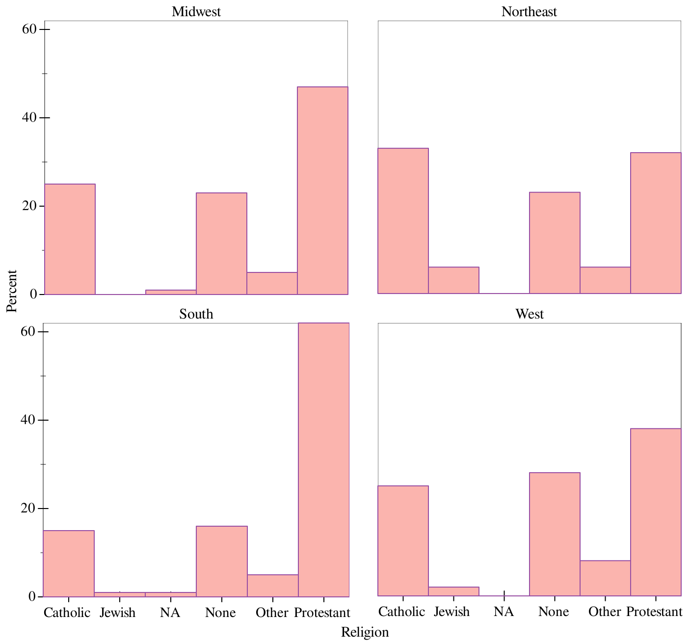
Voilà.

1	Deciding what library to use
2	Key forms
3	Gapminder
4	Bar charts
5	Faceting
6	Data wrangling, 101
7	Data wrangling, 201: Wrangle harder