7 Data wrangling, 201: Wrangle harder

7 Data wrangling, 201: Wrangle harder🔗ℹ

This section of the tutorial is based off of R for Data Science Chapter 12, by Hadley Wickham.

The Sawzall API in this section is not finalized. There are no guarantees about backwards compatibility.

Graphite, and the majority of Sawzall’s operations, assume three things about the data:

Each variable has its own column.
Each observation has its own row.
Each value has its own cell.

This style of presentation is called "tidy data" (hence the name "tidyverse", the R software collection Graphite and Sawzall are inspired by). Data that does not satisfy these properties is called "untidy data", and the process of transforming it into tidy data is called "tidying".

Unfortunately, the overwhelming majority of data that you will encounter in the real world™ is untidy. Most data is managed through spreadsheet software like Excel, and is optimized for data entry, not analysis or visualization.

Let’s take a look at some untidy data. In particular, we’re going to look at tuberculosis data broken down by country, year, age, gender, and diagnosis method. This data comes from the 2014 World Health Organization Global Tuberculosis Report.

> (define who (df-read/csv "data/who.csv" #:na "NA"))
> (df-del-series! who "")
> (show who)
data-frame: 7240 rows x 60 columns
┌────────────┬────────────┬────────────┬───────────┬──────────┬────────────┐
│new_ep_f4554│new_ep_f3544│new_sp_m3544│new_sp_f014│new_sp_f65│new_sn_m3544│
├────────────┼────────────┼────────────┼───────────┼──────────┼────────────┤
│#f          │#f          │#f          │#f         │#f        │#f          │
├────────────┼────────────┼────────────┼───────────┼──────────┼────────────┤
│#f          │#f          │#f          │#f         │#f        │#f          │
├────────────┼────────────┼────────────┼───────────┼──────────┼────────────┤
│#f          │#f          │#f          │#f         │#f        │#f          │
├────────────┼────────────┼────────────┼───────────┼──────────┼────────────┤
│#f          │#f          │#f          │#f         │#f        │#f          │
├────────────┼────────────┼────────────┼───────────┼──────────┼────────────┤
│#f          │#f          │#f          │#f         │#f        │#f          │
├────────────┼────────────┼────────────┼───────────┼──────────┼────────────┤
│#f          │#f          │#f          │#f         │#f        │#f          │
└────────────┴────────────┴────────────┴───────────┴──────────┴────────────┘
7234 rows, 54 cols elided
(use (show df everything #:n-rows 'all) for full frame)
> (df-series-names who)
'("new_ep_f4554"
  "new_ep_f3544"
  "new_sp_m3544"
  "new_sp_f014"
  "new_sp_f65"
  "new_sn_m3544"
  "new_ep_f65"
  "newrel_f5564"
  "newrel_f1524"
  "iso2"
  "country"
  "new_sn_m65"
  "new_sn_f5564"
  "newrel_m1524"
  "new_ep_f1524"
  "newrel_m4554"
  "new_ep_m5564"
  "new_sp_f1524"
  "new_sn_m5564"
  "newrel_m65"
  "new_ep_f5564"
  "new_ep_m1524"
  "newrel_f014"
  "iso3"
  "new_sp_f2534"
  "new_ep_m4554"
  "new_sp_f3544"
  "new_ep_m014"
  "new_sp_m65"
  "new_ep_m2534"
  "newrel_f4554"
  "new_sp_m5564"
  "new_ep_f014"
  "new_sn_f65"
  "new_sp_m2534"
  "new_sn_m014"
  "new_sn_m2534"
  "new_sn_f2534"
  "new_sp_m014"
  "new_sp_f4554"
  "new_ep_f2534"
  "new_sn_f014"
  "new_sp_m1524"
  "year"
  "new_sp_f5564"
  "newrel_m5564"
  "newrel_f65"
  "new_sn_f3544"
  "new_sn_m4554"
  "new_sn_f1524"
  "new_sn_f4554"
  "new_sn_m1524"
  "new_sp_m4554"
  "new_ep_m3544"
  "newrel_m014"
  "newrel_f2534"
  "newrel_m2534"
  "newrel_m3544"
  "new_ep_m65"
  "newrel_f3544")

We remove the empty column because it’s a column of IDs, which is irrelevant for our purposes.

Anyway, wow. Ouch. This is a pretty typical dataset: it has redundant columns, weird variable codes, and missing values abound. Chances are, it was made in spreadsheet software. So, we’ll need multiple steps to try and tidy it.

Here’s a breakdown of what we can deduce for now:

country, iso2, and iso3 are variables that specify the country, the latter two being country codes. We don’t need the latter two, then.
year is clearly a variable.
Given names like newrel_f65 and new_ep_f4554, we can reasonably infer that these are values of some mega-variable.

So, what we want to do is take the names of each new..., and the values of each of those columns, and turn them into two columns: one representing the former name of the column, and one representing the value. Sawzall provides an operation for turning column names that are actually values into a new column: pivot-longer.

To use pivot-longer, we need three things: the set of columns whose names are values and not variables (in this case, everything starting with new), a name of a variable to move the column names to (in this case, key, since we don’t know what these names mean yet), and a name of a variable to move the column values to (we know it’s TB cases, so we’ll call it cases).

So, that looks something like this:

> (~> who
      (pivot-longer (starting-with "new")
                    #:names-to "key"
                    #:values-to "cases")
      show)
data-frame: 405440 rows x 6 columns
┌────┬────────────┬────┬───────────┬─────┬────┐
│year│key         │iso2│country    │cases│iso3│
├────┼────────────┼────┼───────────┼─────┼────┤
│1980│new_ep_f4554│AF  │Afghanistan│#f   │AFG │
├────┼────────────┼────┼───────────┼─────┼────┤
│1981│new_ep_f4554│AF  │Afghanistan│#f   │AFG │
├────┼────────────┼────┼───────────┼─────┼────┤
│1982│new_ep_f4554│AF  │Afghanistan│#f   │AFG │
├────┼────────────┼────┼───────────┼─────┼────┤
│1983│new_ep_f4554│AF  │Afghanistan│#f   │AFG │
├────┼────────────┼────┼───────────┼─────┼────┤
│1984│new_ep_f4554│AF  │Afghanistan│#f   │AFG │
├────┼────────────┼────┼───────────┼─────┼────┤
│1985│new_ep_f4554│AF  │Afghanistan│#f   │AFG │
└────┴────────────┴────┴───────────┴─────┴────┘
405434 rows, 0 cols elided
(use (show df everything #:n-rows 'all) for full frame)

We now have significantly fewer columns, and way more rows, since we transformed all of those messy columns into two. Note the (starting-with "new"): this is a slice spec, a domain-specific language for selecting columns from data. See slice’s documentation for more details.

We can also assume that rows where there are no entered data (so, #f is in them) are irrelevant. To get rid of them, we can use drop-na, which does what it says on the tin:

> (~> who
      (pivot-longer (starting-with "new")
                    #:names-to "key"
                    #:values-to "cases")
      (drop-na "cases")
      show)
data-frame: 76046 rows x 6 columns
┌────┬────┬────────────┬───────┬─────┬────┐
│year│iso2│key         │country│cases│iso3│
├────┼────┼────────────┼───────┼─────┼────┤
│2006│AL  │new_ep_f4554│Albania│12   │ALB │
├────┼────┼────────────┼───────┼─────┼────┤
│2007│AL  │new_ep_f4554│Albania│13   │ALB │
├────┼────┼────────────┼───────┼─────┼────┤
│2008│AL  │new_ep_f4554│Albania│12   │ALB │
├────┼────┼────────────┼───────┼─────┼────┤
│2009│AL  │new_ep_f4554│Albania│8    │ALB │
├────┼────┼────────────┼───────┼─────┼────┤
│2010│AL  │new_ep_f4554│Albania│4    │ALB │
├────┼────┼────────────┼───────┼─────┼────┤
│2011│AL  │new_ep_f4554│Albania│12   │ALB │
└────┴────┴────────────┴───────┴─────┴────┘
76040 rows, 0 cols elided
(use (show df everything #:n-rows 'all) for full frame)

Annoyingly, we don’t understand what key is supposed to mean. Luckily, I’m basing this tutorial off other people’s work, who have conveniently provided the information for me. So, here’s the anatomy of, for example, "new_ep_f4554":

The first three letters are either new or old, denoting new or old cases of TB. We don’t have any old cases in the provided data. So, in this case, we have a new case
The next two letters denote the type of TB:
- rel stands for relapse
- ep stands for extrapulmonary TB (this case)
- sn stands for pulmonary TB that could not be diagnosed by a pulmonary smear (smear negative)
- sp stands for pulmonary TB that could be diagnosed by a pulmonary smear (smear positive)
The sixth letter gives the sex of the patient, either m or f for male and female, respectively.
The remaining numbers give an age group. For example, 014 is 0-14 years old, 4554 is 45-54 years old, and 65 is 65+.

Unfortunately, the cases of relapse are formatted like newrel_f65. So, we’ll use create to replace all instances of "newrel" with "new_rel", so we have a common baseline to split our variable on. Note that binding the variable and making a new column with the same name replaces the old one:

> (~> who
      (pivot-longer (starting-with "new")
                    #:names-to "key"
                    #:values-to "cases")
      (drop-na "cases")
      (create [key (key) (string-replace key "newrel" "new_rel")])
      show)
data-frame: 76046 rows x 6 columns
┌────┬────────────┬────┬───────┬─────┬────┐
│year│key         │iso2│country│cases│iso3│
├────┼────────────┼────┼───────┼─────┼────┤
│2006│new_ep_f4554│AL  │Albania│12   │ALB │
├────┼────────────┼────┼───────┼─────┼────┤
│2007│new_ep_f4554│AL  │Albania│13   │ALB │
├────┼────────────┼────┼───────┼─────┼────┤
│2008│new_ep_f4554│AL  │Albania│12   │ALB │
├────┼────────────┼────┼───────┼─────┼────┤
│2009│new_ep_f4554│AL  │Albania│8    │ALB │
├────┼────────────┼────┼───────┼─────┼────┤
│2010│new_ep_f4554│AL  │Albania│4    │ALB │
├────┼────────────┼────┼───────┼─────┼────┤
│2011│new_ep_f4554│AL  │Albania│12   │ALB │
└────┴────────────┴────┴───────┴─────┴────┘
76040 rows, 0 cols elided
(use (show df everything #:n-rows 'all) for full frame)

Then, we want to split up each variable along the separator "_", pulling apart each value of key into three variables: new, type, and sex-age (since, for example, "f4554") is both the sex and age variable). Sawzall provides the separate function for this purpose:

> (~> who
      (pivot-longer (starting-with "new")
                    #:names-to "key"
                    #:values-to "cases")
      (drop-na "cases")
      (create [key (key) (string-replace key "newrel" "new_rel")])
      (separate "key" #:into '("new" "type" "sex-age") #:separator "_")
      (show ["country" "new" "type" "sex-age"]))
data-frame: 76046 rows x 8 columns
┌───────┬───┬────┬───────┐
│country│new│type│sex-age│
├───────┼───┼────┼───────┤
│Albania│new│ep  │f4554  │
├───────┼───┼────┼───────┤
│Albania│new│ep  │f4554  │
├───────┼───┼────┼───────┤
│Albania│new│ep  │f4554  │
├───────┼───┼────┼───────┤
│Albania│new│ep  │f4554  │
├───────┼───┼────┼───────┤
│Albania│new│ep  │f4554  │
├───────┼───┼────┼───────┤
│Albania│new│ep  │f4554  │
└───────┴───┴────┴───────┘
76040 rows, 4 cols elided
(use (show df everything #:n-rows 'all) for full frame)

The #:into keyword argument determines what column names to split the variable into, and #:separator determines a string to split each value on. Also note how show also takes a slice-spec, so we can determine what columns we want to show.

We have some useless variables now. Namely, new is just "new" repeated over and over, and iso2 and iso3 are country codes, which are irrelevant for our purposes. We can use the slice operator, alongside a slice-spec that takes everything aside from these variables, to remove them from the data:

> (~> who
      (pivot-longer (starting-with "new")
                    #:names-to "key"
                    #:values-to "cases")
      (drop-na "cases")
      (create [key (key) (string-replace key "newrel" "new_rel")])
      (separate "key" #:into '("new" "type" "sex-age") #:separator "_")
      (slice (not ["new" "iso2" "iso3"]))
      show)
data-frame: 76046 rows x 5 columns
┌────┬────┬───────┬─────┬───────┐
│type│year│country│cases│sex-age│
├────┼────┼───────┼─────┼───────┤
│ep  │2006│Albania│12   │f4554  │
├────┼────┼───────┼─────┼───────┤
│ep  │2007│Albania│13   │f4554  │
├────┼────┼───────┼─────┼───────┤
│ep  │2008│Albania│12   │f4554  │
├────┼────┼───────┼─────┼───────┤
│ep  │2009│Albania│8    │f4554  │
├────┼────┼───────┼─────┼───────┤
│ep  │2010│Albania│4    │f4554  │
├────┼────┼───────┼─────┼───────┤
│ep  │2011│Albania│12   │f4554  │
└────┴────┴───────┴─────┴───────┘
76040 rows, 0 cols elided
(use (show df everything #:n-rows 'all) for full frame)

Finally, we can seperate the sex-age variable into two variables, sex and age, with the #:separator 1 – we can specify a number, in which case the variable will be split at this character index.

> (~> who
      (pivot-longer (starting-with "new")
                    #:names-to "key"
                    #:values-to "cases")
      (drop-na "cases")
      (create [key (key) (string-replace key "newrel" "new_rel")])
      (separate "key" #:into '("new" "type" "sex-age") #:separator "_")
      (slice (not ["new" "iso2" "iso3"]))
      (separate "sex-age" #:into '("sex" "age") #:separator 1)
      show)
data-frame: 76046 rows x 6 columns
┌────┬───────┬────┬─────┬────┬───┐
│year│country│type│cases│age │sex│
├────┼───────┼────┼─────┼────┼───┤
│2006│Albania│ep  │12   │4554│f  │
├────┼───────┼────┼─────┼────┼───┤
│2007│Albania│ep  │13   │4554│f  │
├────┼───────┼────┼─────┼────┼───┤
│2008│Albania│ep  │12   │4554│f  │
├────┼───────┼────┼─────┼────┼───┤
│2009│Albania│ep  │8    │4554│f  │
├────┼───────┼────┼─────┼────┼───┤
│2010│Albania│ep  │4    │4554│f  │
├────┼───────┼────┼─────┼────┼───┤
│2011│Albania│ep  │12   │4554│f  │
└────┴───────┴────┴─────┴────┴───┘
76040 rows, 0 cols elided
(use (show df everything #:n-rows 'all) for full frame)

Finally, we have some tidy data! Let’s save it:

> (define tidy-who
    (~> who
        (pivot-longer (starting-with "new")
                      #:names-to "key"
                      #:values-to "cases")
        (drop-na "cases")
        (create [key (key) (string-replace key "newrel" "new_rel")])
        (separate "key" #:into '("new" "type" "sex-age") #:separator "_")
        (slice (not ["new" "iso2" "iso3"]))
        (separate "sex-age" #:into '("sex" "age") #:separator 1)))

Now that we finally have some tidy data, we can make some nice looking plots. Let’s turn this into a plot of TB cases in Afghanistan. We want to use where in order to "filter" down this data into just cases for Afghanistan:

> (~> tidy-who
      (where (country) (string=? country "Afghanistan"))
      show)
data-frame: 244 rows x 6 columns
┌────┬────┬────┬───────────┬─────┬───┐
│year│age │type│country    │cases│sex│
├────┼────┼────┼───────────┼─────┼───┤
│1997│3544│sp  │Afghanistan│3    │m  │
├────┼────┼────┼───────────┼─────┼───┤
│1998│3544│sp  │Afghanistan│90   │m  │
├────┼────┼────┼───────────┼─────┼───┤
│1999│3544│sp  │Afghanistan│47   │m  │
├────┼────┼────┼───────────┼─────┼───┤
│2000│3544│sp  │Afghanistan│149  │m  │
├────┼────┼────┼───────────┼─────┼───┤
│2001│3544│sp  │Afghanistan│274  │m  │
├────┼────┼────┼───────────┼─────┼───┤
│2002│3544│sp  │Afghanistan│368  │m  │
└────┴────┴────┴───────────┴─────┴───┘
238 rows, 0 cols elided
(use (show df everything #:n-rows 'all) for full frame)

where works similarly to each clause of create or aggregate – we bind the variable country as an element, and then filter the rows of the data-frame for those where the body returns true.

Then, if we try to plot this stratified by age, we run into an issue:

> (~> tidy-who
      (where (country) (string=? country "Afghanistan"))
      (graph #:data _
             #:mapping (aes #:x "year" #:y "cases" #:discrete-color "age")
             (lines)))

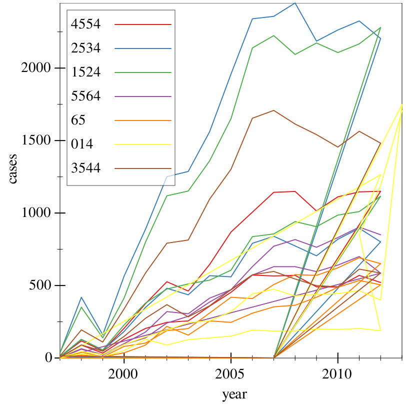
This is a giant mess! The issue is the sex variable – Graphite doesn’t know what to do with this information, since you end up with multiple data-points for year/case. So, we want to group by year and age, sum the case data within them, and then ungroup: this effectively eliminates the sex variable.

> (~> tidy-who
      (where (country) (string=? country "Afghanistan"))
      (group-with "year" "age")
      (aggregate [cases (cases) (sum cases)])
      ungroup
      (graph #:data _
             #:mapping (aes #:x "year" #:y "cases" #:discrete-color "age")
             (lines)))

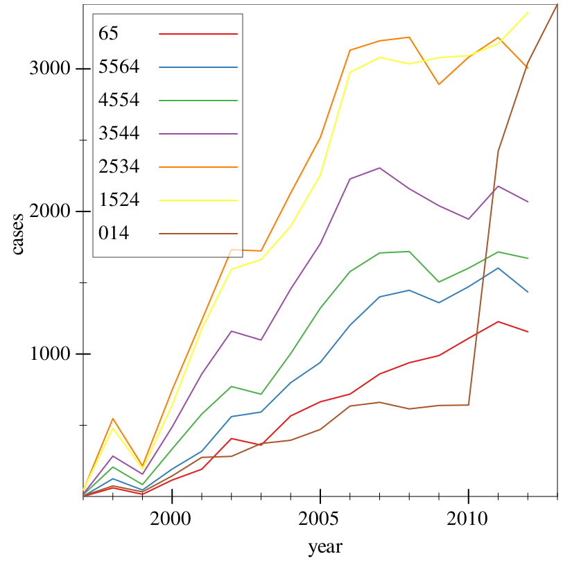
Finally, we have a plot, and we can determine that Afghanistan had a sudden spike in TB cases among ages 0-14 in 2010-2013.

1	Deciding what library to use
2	Key forms
3	Gapminder
4	Bar charts
5	Faceting
6	Data wrangling, 101
7	Data wrangling, 201: Wrangle harder